As we begin a stochastic modeling endeavor to project death claims from a fully underwritten term life insurance portfolio, we first must determine the stochastic method and its components.
Stochastic models typically incorporate Monte Carlo simulation as the method to reflect complex stochastic variable interactions in which alternative analytic approaches would be either unworkable or untenable at best. For the illustrative projection discussed in this article, we developed a Monte Carlo simulation model to stochastically project 30 years of annual claims on a large fully underwritten term life insurance portfolio. We implemented the process in four high-level steps:
- Input variable analysis and specification
- Random sampling of input stochastic variables
- Computation of death benefit projections
- Aggregation and analysis of results
Input Variable Specification
We define input variables as either stochastic or deterministic. Deterministic variables are assigned a predetermined fixed value or may be the result of a fixed non-random formula. Stochastic input variables are assigned statistical distributions and may correlate with other stochastic variables.
In our model, we defined three stochastic input variables: base mortality rate, mortality improvement rate and catastrophic mortality rate. We also defined one deterministic variable: policy lapse rate.
Deterministic Policy Lapse Rate Variable
We could have modeled policy lapse rates stochastically based upon some real-world model of policyholder behavior. However, determining appropriate statistical distributions and correlations for our particular project proved to be difficult: the policyholder’s decision to lapse term insurance typically is not driven by external fluctuating forces such as interest rates or stock market indices, but by other less tractable criteria.
We chose instead to use predetermined best-estimate lapse rates in the Monte Carlo simulation to lapse individual policies randomly (see “Lapse Rates in a Principles-Based World” from the June 2007 Messenger).
Stochastic Base Mortality Variable
This stochastic variable reflects the uncertainty in determining an underlying best-estimate mortality assumption for our portfolio. For this exercise, we referenced a recent mortality experience study for the portfolio. We can think of a mortality study as one random sample from the portfolio’s “true” mortality. Just as with any random sample, uncertainty exists as to whether the sample is a good representation of the population. The uncertainty about a particular study’s credibility is a function of the expected claim count, with uncertainty decreasing as the count increases.
We can model this uncertainty stochastically. With mortality as a binomial process, the experience study’s overall mortality is our mean assumption and 1 / √(#claims) is an approximation of its standard deviation. Then, for a given stochastic iteration, we used the Normal approximation to the Binomial to randomly select a base mortality assumption for that iteration (see“Credibility Analysis for Mortality Experience Studies – Part 1” from the March 2008 Messenger).
Stochastic Mortality Improvement Rate Variable
In our model, mortality improves as we project our portfolio into the future. However, just as with base mortality, uncertainty surrounds the rate at which this improvement will occur. We calculated long-term mean improvement rates, along with corresponding standard deviations, based upon an analysis of US population mortality.
We reviewed historical trends over the past 20-30 years to select appropriate periods for the analysis (Figure 1). A significant and seemingly permanent change in mortality patterns occurred around 1982, so we used data from only 1982 to 2007 in our analysis. For this period, we determined that trended mortality had an annualized mean improvement rate of 0.8 percent with a standard deviation of approximately 0.4 percent.
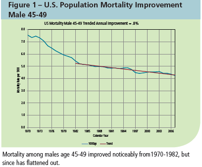
Mortality improvement rates vary significantly by attained age, so we created a vector of improvement assumptions by age group. Recognizing that mortality improvement is correlated among age groups, we also determined a correlation matrix reflecting historical correlations in improvement rates.
Using US population data, we determined that a Normal distribution best represented the fluctuation of improvement rates around the long-term mean. Given the mean and standard deviation parameters, we stochastically generated 10,000 mortality improvement rate scenarios by attained-age group across the projection horizon. We then randomly selected a single scenario from these 10,000 scenarios for application in a single stochastic projection iteration of the portfolio.
Stochastic Catastrophic Mortality Variable
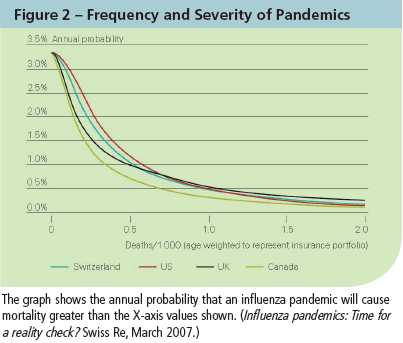
Unlike the property/casualty sector, we are concerned only about catastrophes that result in significant loss of life. Natural disasters were less impactful than pandemics and other disasters which have the potential for loss of life in far greater numbers.
Our model includes a stochastic variable representing additional lives lost in a given calendar year from three types of disasters: pandemics, earthquakes and terrorist attacks. From third-party data sources we developed frequency and severity distributions for each of these types of disasters and randomly sampled these distributions for each projection year (Figure 2).
For each projection year, we randomly sampled the additional catastrophic mortality rate and added this rate to the base mortality of each individual life.
In the next issue we will show how these variables are used and how to analyze the results.